library(foreign)   #for reading dbf files
library(tidyverse) #for data handling, pipes and visualisation
library(readxl)    #for data import directly from Excel
library(janitor) #for unified, easy-to-handle format of variable namesTurboveg to R
The aim of this tutorial is to show you step by step how to import the data from Turboveg 2 to R and prepare it for further analyses.
1.1 Turboveg data format
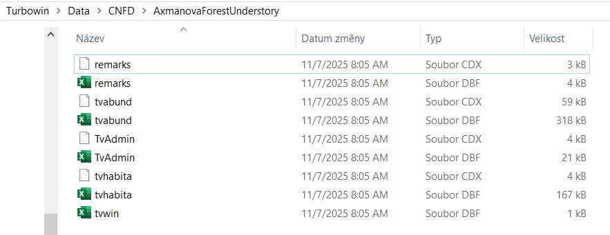
Turboveg for Windows is a program designed for the storage, selection, and export of vegetation plot data (relevés). The data are divided among several files that are matched by either species ID or relevé ID. You do not see this structure directly in the Turboveg interface, but you can find it in the Turbowin folder, subfolder data and particular database (see example below).
At some point, you need to export the data and process them further. This can be done in a specialised software called JUICE, but also directly in R.
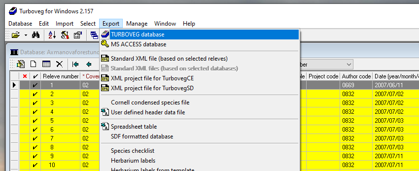
To get Turboveg data to R, you first need to export the Turboveg database to a folder where you want to process the data. This step requires the selection of all the plots you want to export. Alternatively, you can access the files directly in the data folder in Turbowin, but if you do something wrong here, you might completely lose your data.
1.2 Load libraries
1.3 Import env file = header data
1.3.1 Import
One option is to check the exported database manually, open the file called tvhabita.dbf in Excel and save it as tvhabita.xlsx or tvhabita.csv (UTF 8 encoded) file into your data folder. Although it includes one more step outside R, it is still rather straightforward and it saves you troubles with different formats in Turboveg and in R (encoding issues).
You can then import the file from Excel
env <- read_excel("data/tvhabita.xlsx")or from a csv file, which is a slightly more universal option, and we will use it for the import of most of the files.
env <- read_csv("data/tvhabita.csv")Rows: 137 Columns: 84
── Column specification ────────────────────────────────────────────────────────
Delimiter: ","
chr (13): COUNTRY, COVERSCALE, AUTHOR, SYNTAXON, MOSS_IDENT, LICH_IDENT, REM...
dbl (45): RELEVE_NR, DATE, SURF_AREA, ALTITUDE, EXPOSITION, INCLINATIO, COV_...
lgl (26): REFERENCE, TABLE_NR, NR_IN_TAB, PROJECT, UTM, RESURVEY, FOR_EVA, R...
ℹ Use `spec()` to retrieve the full column specification for this data.
ℹ Specify the column types or set `show_col_types = FALSE` to quiet this message.If you check the imported names, they are rather difficult to handle.
names(env) [1] "RELEVE_NR" "COUNTRY" "REFERENCE" "TABLE_NR" "NR_IN_TAB"
[6] "COVERSCALE" "PROJECT" "AUTHOR" "DATE" "SYNTAXON"
[11] "SURF_AREA" "UTM" "ALTITUDE" "EXPOSITION" "INCLINATIO"
[16] "COV_TOTAL" "COV_TREES" "COV_SHRUBS" "COV_HERBS" "COV_MOSSES"
[21] "COV_LICHEN" "COV_ALGAE" "COV_LITTER" "COV_WATER" "COV_ROCK"
[26] "TREE_HIGH" "TREE_LOW" "SHRUB_HIGH" "SHRUB_LOW" "HERB_HIGH"
[31] "HERB_LOW" "HERB_MAX" "CRYPT_HIGH" "MOSS_IDENT" "LICH_IDENT"
[36] "REMARKS" "COORD_CODE" "SYNTAX_OLD" "RESURVEY" "FOR_EVA"
[41] "RS_PROJECT" "RS_SITE" "RS_PLOT" "RS_OBSERV" "PLOT_SHAPE"
[46] "MANIPULATE" "MANIPTYP" "LOC_METHOD" "DATA_OWNER" "EVA_ACCESS"
[51] "LONGITUDE" "LATITUDE" "PRECISION" "LOCALITY" "BIAS_MIN"
[56] "BIAS_GPS" "CEBA_GRID" "FIELD_NR" "HABITAT" "GEOLOGY"
[61] "SOIL" "WATER_PH" "S_PH_H2O" "S_PH_KCL" "S_PH_CACL2"
[66] "SOIL_PH" "CONDUCT" "NR_ORIG" "HLOUBK_CM" "DNO"
[71] "CEL_PLO_M2" "ZAROST_PLO" "ESY_CODE" "ESY_NAME" "COV_WOOD"
[76] "SOIL_DPT" "TRAMPLING" "PLOT_TYPE" "RS_CODE" "RS_PROJTYP"
[81] "RADIATION" "HEAT" "LES" "NELES" Therefore, we will directly change them to tidy names with the clean_names function from the package janitor. An alternative is to rename them one by one using e.g. rename, but here we want to save time and effort.
env <- read_csv("data/tvhabita.csv")%>%
  clean_names()
Rows: 137 Columns: 84
── Column specification ────────────────────────────────────────────────────────
Delimiter: ","
chr (13): COUNTRY, COVERSCALE, AUTHOR, SYNTAXON, MOSS_IDENT, LICH_IDENT, REM...
dbl (45): RELEVE_NR, DATE, SURF_AREA, ALTITUDE, EXPOSITION, INCLINATIO, COV_...
lgl (26): REFERENCE, TABLE_NR, NR_IN_TAB, PROJECT, UTM, RESURVEY, FOR_EVA, R...
ℹ Use `spec()` to retrieve the full column specification for this data.
ℹ Specify the column types or set `show_col_types = FALSE` to quiet this message.tibble(env)# A tibble: 137 × 84
releve_nr country reference table_nr nr_in_tab coverscale project author
<dbl> <chr> <lgl> <lgl> <lgl> <chr> <lgl> <chr>
1 183111 CZ NA NA NA 02 NA 0832
2 183112 CZ NA NA NA 02 NA 0832
3 183113 CZ NA NA NA 02 NA 0832
4 183114 CZ NA NA NA 02 NA 0832
5 183115 CZ NA NA NA 02 NA 0832
6 183116 CZ NA NA NA 02 NA 0832
7 183117 CZ NA NA NA 02 NA 0832
8 183118 CZ NA NA NA 02 NA 0832
9 183119 CZ NA NA NA 02 NA 0832
10 183120 CZ NA NA NA 02 NA 0832
# ℹ 127 more rows
# ℹ 76 more variables: date <dbl>, syntaxon <chr>, surf_area <dbl>, utm <lgl>,
# altitude <dbl>, exposition <dbl>, inclinatio <dbl>, cov_total <dbl>,
# cov_trees <dbl>, cov_shrubs <dbl>, cov_herbs <dbl>, cov_mosses <dbl>,
# cov_lichen <dbl>, cov_algae <dbl>, cov_litter <dbl>, cov_water <dbl>,
# cov_rock <dbl>, tree_high <dbl>, tree_low <dbl>, shrub_high <dbl>,
# shrub_low <dbl>, herb_high <dbl>, herb_low <dbl>, herb_max <dbl>, …Note that the pipe %>% allows the output of a previous command to be used as input to another command instead of using nested functions. It means that a pipe binds individual steps into a sequence and it reads from left to right. You can insert it into your code using Ctrl+Shift+M.
names(env) [1] "releve_nr" "country" "reference" "table_nr" "nr_in_tab"
[6] "coverscale" "project" "author" "date" "syntaxon"
[11] "surf_area" "utm" "altitude" "exposition" "inclinatio"
[16] "cov_total" "cov_trees" "cov_shrubs" "cov_herbs" "cov_mosses"
[21] "cov_lichen" "cov_algae" "cov_litter" "cov_water" "cov_rock"
[26] "tree_high" "tree_low" "shrub_high" "shrub_low" "herb_high"
[31] "herb_low" "herb_max" "crypt_high" "moss_ident" "lich_ident"
[36] "remarks" "coord_code" "syntax_old" "resurvey" "for_eva"
[41] "rs_project" "rs_site" "rs_plot" "rs_observ" "plot_shape"
[46] "manipulate" "maniptyp" "loc_method" "data_owner" "eva_access"
[51] "longitude" "latitude" "precision" "locality" "bias_min"
[56] "bias_gps" "ceba_grid" "field_nr" "habitat" "geology"
[61] "soil" "water_ph" "s_ph_h2o" "s_ph_kcl" "s_ph_cacl2"
[66] "soil_ph" "conduct" "nr_orig" "hloubk_cm" "dno"
[71] "cel_plo_m2" "zarost_plo" "esy_code" "esy_name" "cov_wood"
[76] "soil_dpt" "trampling" "plot_type" "rs_code" "rs_projtyp"
[81] "radiation" "heat" "les" "neles" Pipe also enables us to see the output before saving the result. We want to select just a few variables for checking, but not overwrite the data, before we are happy with the selection. For example, here we see that the habitat information is not filled (returns NAs), so I will not use it.
env %>%
  select(releve_nr, habitat, latitude, longitude)
# A tibble: 137 × 4
releve_nr habitat latitude longitude
<dbl> <lgl> <dbl> <dbl>
1 183111 NA 492015. 163420
2 183112 NA 492129. 163346.
3 183113 NA 492126. 162913.
4 183114 NA 490210. 162138.
5 183115 NA 490203. 162128.
6 183116 NA 490158. 162117.
7 183117 NA 490253. 162349.
8 183118 NA 490730. 161735.
9 183119 NA 490742. 161622.
10 183120 NA 490814. 161507
# ℹ 127 more rowsWhen I am fine with the selection, I can rewrite the file
env <- env %>%
  select(releve_nr, coverscale,field_nr, country, author, date, syntaxon,
         altitude, exposition, inclinatio,
         cov_trees, cov_shrubs, cov_herbs, cov_mosses,
         latitude, longitude, precision, bias_min, bias_gps, locality )
Or I can add all the steps I did so far into one pipeline and check the resulting dataset
env <- read_csv("data/tvhabita.csv")%>%
  clean_names() %>%
  select(releve_nr, coverscale, field_nr, country, author, date, syntaxon,
         altitude, exposition, inclinatio,
         cov_trees, cov_shrubs, cov_herbs, cov_mosses,
         latitude, longitude, precision, bias_min, bias_gps, locality ) %>%
  glimpse()
Rows: 137 Columns: 84
── Column specification ────────────────────────────────────────────────────────
Delimiter: ","
chr (13): COUNTRY, COVERSCALE, AUTHOR, SYNTAXON, MOSS_IDENT, LICH_IDENT, REM...
dbl (45): RELEVE_NR, DATE, SURF_AREA, ALTITUDE, EXPOSITION, INCLINATIO, COV_...
lgl (26): REFERENCE, TABLE_NR, NR_IN_TAB, PROJECT, UTM, RESURVEY, FOR_EVA, R...
ℹ Use `spec()` to retrieve the full column specification for this data.
ℹ Specify the column types or set `show_col_types = FALSE` to quiet this message.Rows: 137
Columns: 20
$ releve_nr <dbl> 183111, 183112, 183113, 183114, 183115, 183116, 183117, 183…
$ coverscale <chr> "02", "02", "02", "02", "02", "02", "02", "02", "02", "02",…
$ field_nr <chr> "2/2007", "3/2007", "4/2007", "5/2007", "6/2007", "7/2007",…
$ country <chr> "CZ", "CZ", "CZ", "CZ", "CZ", "CZ", "CZ", "CZ", "CZ", "CZ",…
$ author <chr> "0832", "0832", "0832", "0832", "0832", "0832", "0832", "08…
$ date <dbl> 20070702, 20070702, 20070702, 20070703, 20070703, 20070703,…
$ syntaxon <chr> "LDA01", "LDA01", "LDA", "LDA01", "LDA", "LD", "LBB", "LB",…
$ altitude <dbl> 458, 414, 379, 374, 380, 373, 390, 255, 340, 368, 356, 427,…
$ exposition <dbl> 150, 150, 210, NA, 170, 65, NA, 80, 220, 95, 200, 170, 130,…
$ inclinatio <dbl> 24, 13, 21, 0, 10, 6, 0, 38, 13, 29, 38, 27, 7, 22, 9, 21, …
$ cov_trees <dbl> 80, 80, 75, 70, 65, 65, 85, 80, 70, 85, 45, 70, 65, 70, 80,…
$ cov_shrubs <dbl> 0, 0, 0, 0, 1, 0, 0, 20, 0, 15, 1, 0, 2, 1, 12, 0, 0, 0, 0,…
$ cov_herbs <dbl> 25, 25, 30, 35, 60, 70, 70, 15, 75, 8, 75, 40, 60, 40, 60, …
$ cov_mosses <dbl> 10, 8, 10, 8, 3, 5, 5, 10, 3, 5, 20, 3, 5, 30, 1, 5, 1, 5, …
$ latitude <dbl> 492015.3, 492128.9, 492126.4, 490210.2, 490203.1, 490158.5,…
$ longitude <dbl> 163420.0, 163345.8, 162913.4, 162137.8, 162128.3, 162117.2,…
$ precision <dbl> 0, 0, 0, 0, 0, 0, 0, 0, 0, 0, 0, 0, 0, 0, 0, 0, 0, 0, 0, 0,…
$ bias_min <dbl> 0, 0, 0, 0, 0, 0, 0, 0, 0, 0, 0, 0, 0, 0, 0, 0, 0, 0, 0, 0,…
$ bias_gps <dbl> 5, 6, 10, 6, 5, 6, 14, 6, 4, 5, 5, 5, 6, 6, 5, 11, 8, 7, 4,…
$ locality <chr> "Svinošice (Brno, Kuřim); 450 m SZ od středu obce", "Lažany…And save it for easier access. Always keep releve_nr and coverscale, as you will need them later.
write.csv(env, "data/env.csv")*An alternative option is to directly import the file exported from the Turboveg database named tvhabita.dbf. Since dbf is a specific type of files and we need to use a specialised packages. Here I used read.dbf function from the foreign library.
env_dbf <- read.dbf("data/tvhabita.dbf", as.is = F) %>%
  clean_names()
Check the structure, directly in R
view(env_dbf)Get the list of the variable names
names(env_dbf) [1] "releve_nr" "country" "reference" "table_nr" "nr_in_tab"
[6] "coverscale" "project" "author" "date" "syntaxon"
[11] "surf_area" "utm" "altitude" "exposition" "inclinatio"
[16] "cov_total" "cov_trees" "cov_shrubs" "cov_herbs" "cov_mosses"
[21] "cov_lichen" "cov_algae" "cov_litter" "cov_water" "cov_rock"
[26] "tree_high" "tree_low" "shrub_high" "shrub_low" "herb_high"
[31] "herb_low" "herb_max" "crypt_high" "moss_ident" "lich_ident"
[36] "remarks" "coord_code" "syntax_old" "resurvey" "for_eva"
[41] "rs_project" "rs_site" "rs_plot" "rs_observ" "plot_shape"
[46] "manipulate" "maniptyp" "loc_method" "data_owner" "eva_access"
[51] "longitude" "latitude" "precision" "locality" "bias_min"
[56] "bias_gps" "ceba_grid" "field_nr" "habitat" "geology"
[61] "soil" "water_ph" "s_ph_h2o" "s_ph_kcl" "s_ph_cacl2"
[66] "soil_ph" "conduct" "nr_orig" "hloubk_cm" "dno"
[71] "cel_plo_m2" "zarost_plo" "esy_code" "esy_name" "cov_wood"
[76] "soil_dpt" "trampling" "plot_type" "rs_code" "rs_projtyp"
[81] "radiation" "heat" "les" "neles" There are several issues with this type of import, as there might be different encodings used in the original files, not compatible with R. For the Czech dataset, I needed to further change the encoding style, so that the diacritics in text columns is translated correctly.
First we need to select the columns that include text and can have issues with diacritics and special symbols, e.g. remarks, locality… I specify them in the brackets and use function iconv to change the encoding to UTF-8. You may need to play a bit to see if it works correctly and change the original type in the from argument. I added one more line to transform the dataframe to tibble, which is the data format used in tidyverse packages.
env_dbf %>%
  mutate(across(c(remarks, locality, habitat, soil),
                ~ iconv(.x, from = "cp852", to = "UTF-8"))) %>%
  select(locality, soil) %>%
  as_tibble()
# A tibble: 137 × 2
locality soil
<chr> <chr>
1 Svinošice (Brno, Kuřim); 450 m SZ od středu obce <NA>
2 Lažany (Brno, Kuřim); 1 km VSV od středu obce <NA>
3 Všechovice (Tišnov); 500 m Z od středu obce <NA>
4 Vedrovice (Moravský Krumlov), Krumlovský les; 2,2 km SZ od středu obce <NA>
5 Vedrovice (Moravský Krumlov), Krumlovský les; 2,1 km SZ od středu obce <NA>
6 Vedrovice (Moravský Krumlov), Krumlovský les; 2,2 km SZ od středu obce <NA>
7 Vedrovice (Moravský Krumlov), Krumlovský les; 3,3 km SSV od středu obce <NA>
8 Čučice (Oslavany), Přírodní park Oslava; 1,7 km JV od středu obce <NA>
9 Čučice (Oslavany), Přírodní park Oslava; 1 km JJZ od středu obce <NA>
10 Senorady (Oslavany), Přírodní park Oslava; 1,2 km SSV od středu obce <NA>
# ℹ 127 more rowsIn the next step we select variables we want to keep further, which is useful, as the database structure also includes predefined variables, even if they are empty. Another advantage of the select function.
env <- env_dbf %>%
  mutate(across(c(remarks, locality, habitat, soil),
                ~ iconv(.x, from = "cp852", to = "UTF-8"))) %>%
  select(releve_nr, coverscale,field_nr, country, author, date, syntaxon,
         altitude, exposition, inclinatio,
         cov_trees, cov_shrubs, cov_herbs, cov_mosses,
         latitude, longitude, precision, bias_min, bias_gps, locality )%>%
  as_tibble()
1.3.2 Coordinates
In the Turboveg 2 databases, the geographical coordinates are stored in a format with DDMMSS.SS. To show the plots in the map or perform any spatial calculations, you will need to transform the coordinates to decimal degrees.

That is the purpose of the following function, where I specify which parts of the string are degrees (position 1-2), which are minutes (3-4) and seconds (5 to11) and how to transform them.
 coord_to_degrees <- function(coord){
  as.numeric(str_sub(coord, 1, 2)) + as.numeric(str_sub(coord, 3, 4)) / 60 + as.numeric(str_sub(coord, 5, 11)) / 3600
}
Below I will check if it works as I need. Please consider that here we apply it to central European dataset and adjustments are needed in other countries e.g. if the coordinates are higher than 99° ~ DDDMMSS.SS
env %>%
  mutate(deg_lat = coord_to_degrees(latitude),
         deg_lon = coord_to_degrees(longitude)) %>%
  select(releve_nr, latitude, deg_lat, longitude, deg_lon)
# A tibble: 137 × 5
releve_nr latitude deg_lat longitude deg_lon
<int> <dbl> <dbl> <dbl> <dbl>
1 183111 492015. 49.3 163420 16.6
2 183112 492129. 49.4 163346. 16.6
3 183113 492126. 49.4 162913. 16.5
4 183114 490210. 49.0 162138. 16.4
5 183115 490203. 49.0 162128. 16.4
6 183116 490158. 49.0 162117. 16.4
7 183117 490253. 49.0 162349. 16.4
8 183118 490730. 49.1 161735. 16.3
9 183119 490742. 49.1 161622. 16.3
10 183120 490814. 49.1 161507 16.3
# ℹ 127 more rowsIf I know I will need coordinates for mapping I will add the respective lines directly to my pipeline
env <- read_csv("data/tvhabita.csv")%>%
  clean_names() %>%
  mutate(deg_lat = coord_to_degrees(latitude),
         deg_lon = coord_to_degrees(longitude)) %>%
  select(releve_nr, coverscale, field_nr, country, author, date, syntaxon,
         altitude, exposition, inclinatio,
         cov_trees, cov_shrubs, cov_herbs, cov_mosses,
         deg_lat, deg_lon, precision, bias_min, bias_gps, locality) %>%
  glimpse()
Rows: 137 Columns: 84
── Column specification ────────────────────────────────────────────────────────
Delimiter: ","
chr (13): COUNTRY, COVERSCALE, AUTHOR, SYNTAXON, MOSS_IDENT, LICH_IDENT, REM...
dbl (45): RELEVE_NR, DATE, SURF_AREA, ALTITUDE, EXPOSITION, INCLINATIO, COV_...
lgl (26): REFERENCE, TABLE_NR, NR_IN_TAB, PROJECT, UTM, RESURVEY, FOR_EVA, R...
ℹ Use `spec()` to retrieve the full column specification for this data.
ℹ Specify the column types or set `show_col_types = FALSE` to quiet this message.Rows: 137
Columns: 20
$ releve_nr <dbl> 183111, 183112, 183113, 183114, 183115, 183116, 183117, 183…
$ coverscale <chr> "02", "02", "02", "02", "02", "02", "02", "02", "02", "02",…
$ field_nr <chr> "2/2007", "3/2007", "4/2007", "5/2007", "6/2007", "7/2007",…
$ country <chr> "CZ", "CZ", "CZ", "CZ", "CZ", "CZ", "CZ", "CZ", "CZ", "CZ",…
$ author <chr> "0832", "0832", "0832", "0832", "0832", "0832", "0832", "08…
$ date <dbl> 20070702, 20070702, 20070702, 20070703, 20070703, 20070703,…
$ syntaxon <chr> "LDA01", "LDA01", "LDA", "LDA01", "LDA", "LD", "LBB", "LB",…
$ altitude <dbl> 458, 414, 379, 374, 380, 373, 390, 255, 340, 368, 356, 427,…
$ exposition <dbl> 150, 150, 210, NA, 170, 65, NA, 80, 220, 95, 200, 170, 130,…
$ inclinatio <dbl> 24, 13, 21, 0, 10, 6, 0, 38, 13, 29, 38, 27, 7, 22, 9, 21, …
$ cov_trees <dbl> 80, 80, 75, 70, 65, 65, 85, 80, 70, 85, 45, 70, 65, 70, 80,…
$ cov_shrubs <dbl> 0, 0, 0, 0, 1, 0, 0, 20, 0, 15, 1, 0, 2, 1, 12, 0, 0, 0, 0,…
$ cov_herbs <dbl> 25, 25, 30, 35, 60, 70, 70, 15, 75, 8, 75, 40, 60, 40, 60, …
$ cov_mosses <dbl> 10, 8, 10, 8, 3, 5, 5, 10, 3, 5, 20, 3, 5, 30, 1, 5, 1, 5, …
$ deg_lat <dbl> 49.33758, 49.35803, 49.35733, 49.03617, 49.03419, 49.03292,…
$ deg_lon <dbl> 16.57222, 16.56272, 16.48706, 16.36050, 16.35786, 16.35478,…
$ precision <dbl> 0, 0, 0, 0, 0, 0, 0, 0, 0, 0, 0, 0, 0, 0, 0, 0, 0, 0, 0, 0,…
$ bias_min <dbl> 0, 0, 0, 0, 0, 0, 0, 0, 0, 0, 0, 0, 0, 0, 0, 0, 0, 0, 0, 0,…
$ bias_gps <dbl> 5, 6, 10, 6, 5, 6, 14, 6, 4, 5, 5, 5, 6, 6, 5, 11, 8, 7, 4,…
$ locality <chr> "Svinošice (Brno, Kuřim); 450 m SZ od středu obce", "Lažany…and save it for later
write.csv(env, "data/env.csv")1.4 Import spe file = species file in a long format
The first option is again to open the tvabund.dbf in Excel, save it as tvabund.csv and import it to our environment in R. Again, I will use the clean_names function during import, so that we have the same style of the variable names.
tvabund <- read_csv("data/tvabund.csv") %>%
  clean_names()
Rows: 4583 Columns: 5
── Column specification ────────────────────────────────────────────────────────
Delimiter: ","
chr (1): COVER_CODE
dbl (3): RELEVE_NR, SPECIES_NR, LAYER
lgl (1): _ORIG_NAME
ℹ Use `spec()` to retrieve the full column specification for this data.
ℹ Specify the column types or set `show_col_types = FALSE` to quiet this message.*An alternative option is to read the data directly from the dbf file. In this case, it is less complicated than the import of an env file, as there are no problematic text variables.
tvabund <- read.dbf("data/tvabund.dbf", as.is = F) %>%
clean_names()glimpse(tvabund)Rows: 4,583
Columns: 5
$ releve_nr <dbl> 183111, 183111, 183111, 183111, 183111, 183111, 183111, 183…
$ species_nr <dbl> 2206, 2315, 3351, 4283, 4430, 4577, 5127, 5137, 5165, 5353,…
$ cover_code <chr> "+", "1", "r", "1", "r", "r", "1", "+", "r", "r", "2b", "+"…
$ layer <dbl> 6, 7, 6, 6, 7, 6, 6, 6, 6, 6, 6, 6, 6, 6, 1, 7, 6, 6, 6, 6,…
$ orig_name <lgl> NA, NA, NA, NA, NA, NA, NA, NA, NA, NA, NA, NA, NA, NA, NA,…Now we will check the data again and we see, that there are no species names, just numbers. Also, the cover is given in the original codes and not in percentages. See the scheme below to understand where each piece of information is stored.
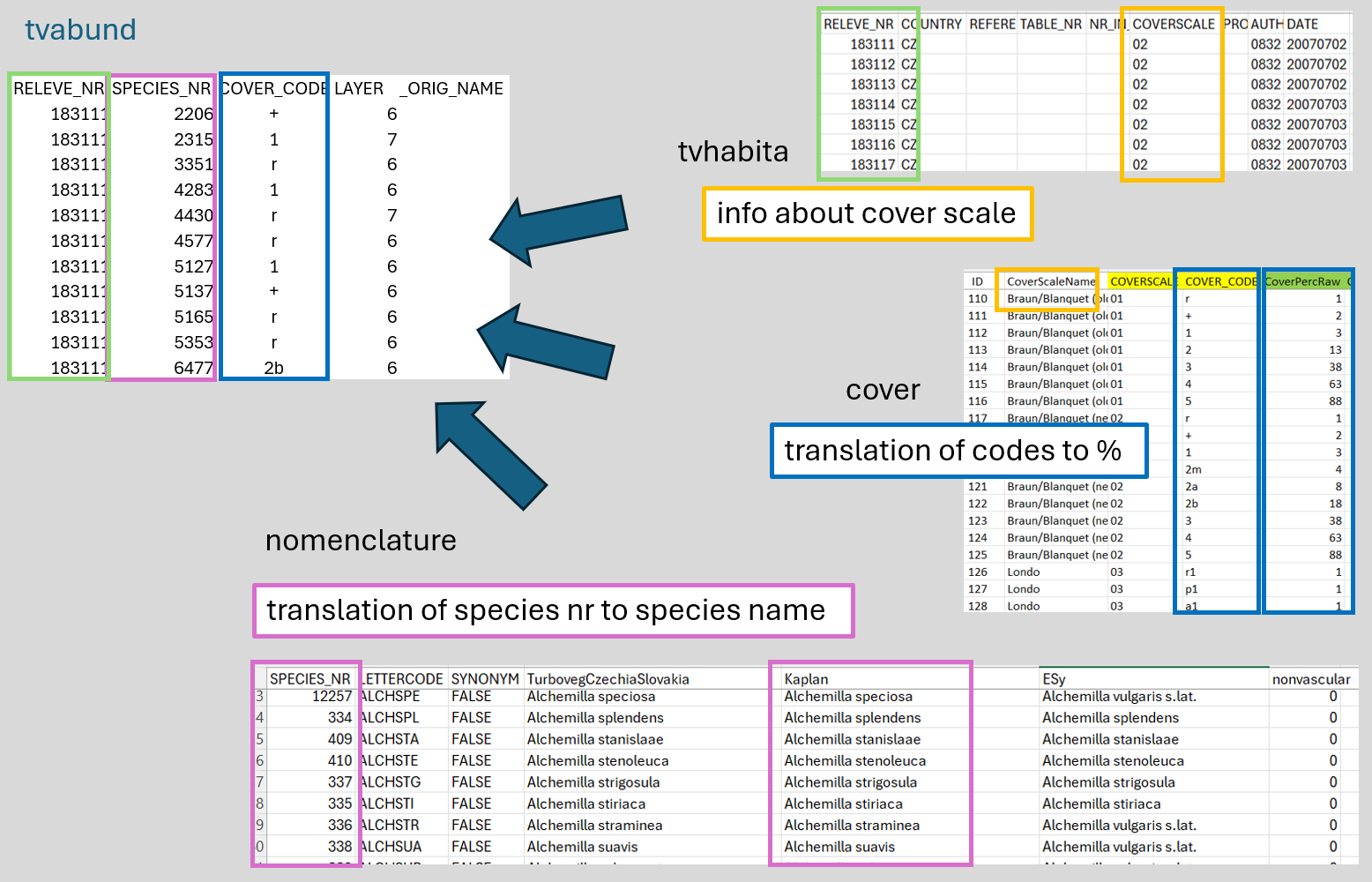
We have to prepare these different files we need, import them and merge them.
1.4.1 Nomenclature
In the abund file, species numbers refer to the codes in the checklist used in the Turboveg database. To translate them into species names you will need a translation table with the original number in the database, the original name in the database and the name you want to use in the analyses.
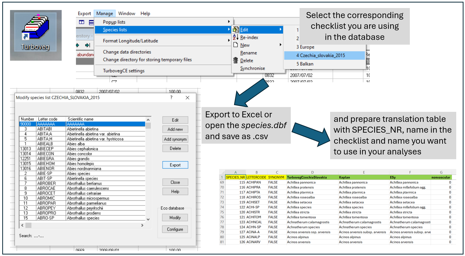
Preparation of the translation table: To show you how to prepare such a table, I opened the checklist file, so called species.dbf from the folder: Turbowin/species/CzechiaSlovakia2015 and saved it here in the data folder as species.csv. Using the following pipeline, you can prepare your own translation table and add other names or information.
nomenclature_raw <- read_csv("data/species.csv") %>%
  clean_names() %>%
  left_join(select(., species_nr, accepted_abbreviat = abbreviat),
            by = c("valid_nr" = "species_nr")) %>%
  mutate(accepted_name = if_else(synonym, accepted_abbreviat, abbreviat)) %>%
  select(-accepted_abbreviat)
Rows: 13863 Columns: 6
── Column specification ────────────────────────────────────────────────────────
Delimiter: ","
chr (3): LETTERCODE, SHORTNAME, ABBREVIAT
dbl (2): SPECIES_NR, VALID_NR
lgl (1): SYNONYM
ℹ Use `spec()` to retrieve the full column specification for this data.
ℹ Specify the column types or set `show_col_types = FALSE` to quiet this message.We will now import the nomenclature file that is already adapted for the Czech flora.
nomenclature <- read_csv("data/nomenclature_20251108.csv") %>%
  clean_names()
Rows: 13862 Columns: 7
── Column specification ────────────────────────────────────────────────────────
Delimiter: ","
chr (4): LETTERCODE, TurbovegCzechiaSlovakia, Kaplan, ExpertSystem
dbl (2): SPECIES_NR, nonvascular
lgl (1): SYNONYM
ℹ Use `spec()` to retrieve the full column specification for this data.
ℹ Specify the column types or set `show_col_types = FALSE` to quiet this message.tibble(nomenclature)# A tibble: 13,862 × 7
species_nr lettercode synonym turboveg_czechia_slovakia kaplan expert_system
<dbl> <chr> <lgl> <chr> <chr> <chr>
1 14321 *CONC*C FALSE x Conygeron huelsenii x Con… x Conyzigero…
2 14323 *DACD*A FALSE x Dactylodenia gracilis x Dac… x Dactylogym…
3 14324 *DACD*A TRUE x Dactylodenia st.-quinti… x Dac… x Dactylogym…
4 14322 *DACD*D FALSE x Dactylodenia comigera x Dac… x Dactylogym…
5 14325 *DATD*D FALSE x Dactyloglossum erdingeri x Dac… x Dactyloglo…
6 14327 *FESF*E FALSE x Festulolium loliaceum x Fes… x Festuloliu…
7 14326 *FESF*F FALSE x Festulolium braunii x Fes… x Festuloliu…
8 14328 *GYMG*G FALSE x Gymnanacamptis anacampt… x Gym… x Gymnanacam…
9 14329 *ORCO*O FALSE x Orchidactyla boudieri x Dac… x Dactylocam…
10 14330 *PSEP*P FALSE x Pseudadenia schweinfurt… x Pse… x Pseudadeni…
# ℹ 13,852 more rows
# ℹ 1 more variable: nonvascular <dbl>There are several advantages of this approach. First, you can adjust the nomenclature to the newest source/regional checklist. In our example, the name in Turboveg is translated to the nomenclature presented in the recent edition of the Key to the Flora of the Czech Republick, and it is named after the main editor Kaplan.
Second, I can add a concept that groups several taxa into higher units, e.g. taxa that are not easy to recognise in the field are assigned into aggregates. This is exactly the same approach you use when creating an expert system file. Here it is even easier to understand and much easier to change the translation when you need to fix something. The name in this file is called ESy.
Last but not least. I can directly add much more information into such a table. For example invasion status, growth form or anything else. Here we have an indication of whether the species is nonvascular.
I might want to check how the species are translated using my translation file and select just these matching rows. Either create a variable called selection indicating if the species is in the subset or not.
nomenclature_check<- nomenclature %>%
  left_join(tvabund %>%
              distinct(species_nr)%>%
              mutate(selection=1))
Joining with `by = join_by(species_nr)`or I can even add the frequency, how many times it appears in the records of the dataset
nomenclature_check<- nomenclature %>%
  left_join(tvabund %>%
              count(species_nr))
Joining with `by = join_by(species_nr)`I can then write the file, make adjustments e.g. in Excel and upload it again. Great thing is that I have an indication of which species are in the dataset, and I do not have to pay attention to the other rows.
write.csv(nomenclature_check, "data/nomenclature_check.csv")upload the new, adjusted file
nomenclature <- read_csv("data/nomenclature_check.csv") %>%
  clean_names()
1.4.2 Cover
We have a translation table for nomenclature, but we still need to translate cover codes to percentages. For translation of cover we need to use information about the cover scale (stored in the header data / tvhabita / env file) and information on how to translate the values in that particular scale to percentages. The file here was prepared based on the translation of cover values in different scales to percentages following the EVA database approach. One more column was added to enable different adjustments, for example, change the values for rare species. For any project, we suggest to open the file and check if the scales you are using are there and if you agree with the translation.
cover <- read_csv("data/cover_20230402.csv") %>% clean_names() Rows: 326 Columns: 6
── Column specification ────────────────────────────────────────────────────────
Delimiter: ","
chr (3): CoverScaleName, COVERSCALE, COVER_CODE
dbl (3): ID, CoverPercEVA, CoverPerc
ℹ Use `spec()` to retrieve the full column specification for this data.
ℹ Specify the column types or set `show_col_types = FALSE` to quiet this message.tibble(cover)# A tibble: 326 × 6
id cover_scale_name coverscale cover_code cover_perc_eva cover_perc
<dbl> <chr> <chr> <chr> <dbl> <dbl>
1 1 Percetage % 00 0.1 0.1 0.1
2 2 Percetage % 00 0.2 0.2 0.2
3 3 Percetage % 00 0.3 0.3 0.3
4 4 Percetage % 00 0.4 0.4 0.4
5 5 Percetage % 00 0.5 0.5 0.5
6 6 Percetage % 00 0.6 0.6 0.6
7 7 Percetage % 00 0.7 0.7 0.7
8 8 Percetage % 00 0.8 0.8 0.8
9 9 Percetage % 00 0.9 0.9 0.9
10 10 Percetage % 00 1 1 1
# ℹ 316 more rowsHere I can check the different scale names included in the file
cover %>% distinct(cover_scale_name) # A tibble: 16 × 1
cover_scale_name
<chr>
1 Percetage %
2 Braun/Blanquet (old)
3 Braun/Blanquet (new)
4 Londo
5 Presence/Absence
6 Ordinale scale (1-9)
7 Barkman, Doing & Segal
8 Doing
9 Domin
10 Sedlakova
11 Zlatnˇk
12 Percentual scale
13 Hedl
14 Kuźera
15 Domin (uprava Hadac)
16 Percentual (r, +) And I can also filter the rows of the specified scales. E.g. here I am looking for all those that start with a specific pattern “Braun”
cover %>%
  filter(str_starts(cover_scale_name, "Braun")) %>%
  print(n=20)
# A tibble: 16 × 6
id cover_scale_name coverscale cover_code cover_perc_eva cover_perc
<dbl> <chr> <chr> <chr> <dbl> <dbl>
1 110 Braun/Blanquet (old) 01 r 1 1
2 111 Braun/Blanquet (old) 01 + 2 2
3 112 Braun/Blanquet (old) 01 1 3 3
4 113 Braun/Blanquet (old) 01 2 13 13
5 114 Braun/Blanquet (old) 01 3 38 38
6 115 Braun/Blanquet (old) 01 4 63 63
7 116 Braun/Blanquet (old) 01 5 88 88
8 117 Braun/Blanquet (new) 02 r 1 0.1
9 118 Braun/Blanquet (new) 02 + 2 0.5
10 119 Braun/Blanquet (new) 02 1 3 3
11 120 Braun/Blanquet (new) 02 2m 4 4
12 121 Braun/Blanquet (new) 02 2a 8 10
13 122 Braun/Blanquet (new) 02 2b 18 20
14 123 Braun/Blanquet (new) 02 3 38 37.5
15 124 Braun/Blanquet (new) 02 4 63 62.5
16 125 Braun/Blanquet (new) 02 5 88 87.51.4.2 Merging all files into complete spe file
Finally, I have translation to nomenclature, to cover, so I need to put everything together.
tvabund %>%
  left_join(nomenclature %>%
              select(species_nr, kaplan, expert_system, nonvascular)) %>%
  left_join(env %>% select(releve_nr, coverscale)) %>%
  left_join(cover %>% select(coverscale,cover_code,cover_perc))
Joining with `by = join_by(species_nr)`
Joining with `by = join_by(releve_nr)`
Joining with `by = join_by(cover_code, coverscale)`# A tibble: 4,583 × 10
releve_nr species_nr cover_code layer orig_name kaplan expert_system
<dbl> <dbl> <chr> <dbl> <lgl> <chr> <chr>
1 183111 2206 + 6 NA Carex digitata… Carex digita…
2 183111 2315 1 7 NA Carpinus betul… Carpinus bet…
3 183111 3351 r 6 NA Cytisus nigric… Cytisus nigr…
4 183111 4283 1 6 NA Festuca ovina Festuca ovina
5 183111 4430 r 7 NA Fraxinus excel… Fraxinus exc…
6 183111 4577 r 6 NA Galium rotundi… Galium rotun…
7 183111 5127 1 6 NA Hieracium lach… Hieracium la…
8 183111 5137 + 6 NA Hieracium muro… Hieracium mu…
9 183111 5165 r 6 NA Hieracium saba… Hieracium sa…
10 183111 5353 r 6 NA Hypericum perf… Hypericum pe…
# ℹ 4,573 more rows
# ℹ 3 more variables: nonvascular <dbl>, coverscale <chr>, cover_perc <dbl>The output contains these variables
"releve_nr" "species_nr" "cover_code" "layer" "orig_name" "kaplan" "expert_system" "nonvascular" "coverscale" "cover_perc" If I am satisfied with the result, I assign the pipeline into the spe file and add one more line to select just the needed variables. Here I decided to use the expert_system name and I renamed it directly in the select function.
spe<- tvabund %>%
  left_join(nomenclature %>%
              select(species_nr, kaplan, expert_system, nonvascular)) %>%
  left_join(env %>% select(releve_nr, coverscale)) %>%
  left_join(cover %>% select(coverscale,cover_code,cover_perc)) %>%
  # filter (!nonvascular=1) %>% # optional to remove nonvasculars
  select(releve_nr, species= expert_system, nonvascular, layer, cover_perc)
Joining with `by = join_by(species_nr)`
Joining with `by = join_by(releve_nr)`
Joining with `by = join_by(cover_code, coverscale)`To see the result we will use view
view(spe)We can again save the final file, to be easily accessible for later
write.csv(spe, "data/spe.csv")1.5 Merging of species covers across layers
1.5.1 Duplicate species records
What is the problem? Sometimes we have some species names listed more than once in the same plot. Either because we changed the original concept (from subspecies to species level, or after additional identification) or because we recorded the same species in different layers. Depending on our further questions and analyses this might become minor or bigger problem.
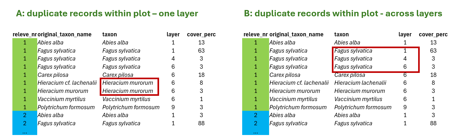
A> In the first case, duplicate within one layer, I can fix the problem by summing the values for the same species in the same layer to get distinct species-layer combinations per plot. This is something we need to do. Otherwise our data would go against tidy approach and we will experience issues in joins, summarisation etc.
B> In the other case, duplicate across layers, the data are OK, because there is one more variable that makes it unique record (layer). But if we want to look at the whole community and e.g. calculate share of some life forms weighted by cover, etc. we again need to sum the values across layers and put all the species as they were in the same layer (this is then usually marked as 0).
1.5.2 Duplicates checking
We recommend to always do the following check of the data. Simply group species by releves/plots and count if some of the species are at more rows.
spe %>%
  group_by(releve_nr, species, layer) %>%
  count() %>%
  filter(n>1)
# A tibble: 2 × 4
# Groups: releve_nr, species, layer [2]
releve_nr species layer n
<dbl> <chr> <dbl> <int>
1 132 Galium palustre agg. 6 2
2 183182 Galium palustre agg. 6 2We can see that in two releves/plots there is a conflict in the species Galium palustre agg. Most probably we separated two species in the field that we later on decided to group into this aggregate. We can go back and check where exactly this happened, by exactly specifying where to look.
tvabund %>%
  select(releve_nr, species_nr)%>%
  left_join(nomenclature %>%
              select(species_nr, turboveg= turboveg_czechia_slovakia,  species=expert_system)) %>%
  filter(releve_nr %in% c(132, 183182) & species =="Galium palustre agg.")
Joining with `by = join_by(species_nr)`# A tibble: 4 × 4
releve_nr species_nr turboveg species
<dbl> <dbl> <chr> <chr>
1 183182 4558 Galium elongatum Galium palustre agg.
2 183182 4570 Galium palustre Galium palustre agg.
3 132 4558 Galium elongatum Galium palustre agg.
4 132 4570 Galium palustre Galium palustre agg.Alternatively, I can save the first output and use semi-join function, which is very useful if there are more rows I want to check and I do not need to specify multiple conditions in the filter.
test<-spe %>%
  group_by(releve_nr, species, layer) %>%
  count() %>%
  filter(n>1)

tvabund %>%
  select(releve_nr, species_nr)%>%
  left_join(nomenclature %>%
              select(species_nr, turboveg= turboveg_czechia_slovakia, species=expert_system)) %>%
  semi_join(test)
Joining with `by = join_by(species_nr)`
Joining with `by = join_by(releve_nr, species)`# A tibble: 4 × 4
releve_nr species_nr turboveg species
<dbl> <dbl> <chr> <chr>
1 183182 4558 Galium elongatum Galium palustre agg.
2 183182 4570 Galium palustre Galium palustre agg.
3 132 4558 Galium elongatum Galium palustre agg.
4 132 4570 Galium palustre Galium palustre agg.OK, I understand why it happened and I have to fix it now. But we continue checking. Now we will check if there is also problem with species across layers (B). I will simply change the grouping conditions, to the higher hierarchy.
spe %>%
  group_by(releve_nr, species) %>%
  count() %>%
  filter(n>1)
# A tibble: 375 × 3
# Groups: releve_nr, species [375]
releve_nr species n
<dbl> <chr> <int>
1 1 Acer campestre 2
2 1 Quercus petraea agg. 2
3 2 Quercus petraea agg. 2
4 3 Quercus petraea agg. 2
5 4 Carpinus betulus 2
6 4 Quercus petraea agg. 2
7 5 Quercus petraea agg. 2
8 6 Ligustrum vulgare 2
9 6 Quercus petraea agg. 2
10 6 Rosa species 2
# ℹ 365 more rowsWe got lot of duplicates, right? But it is understandable in the vegetation type we have. So keep it in mind for later analyses.
Sometimes it is good to take some extra time and just look at what is inside. Are there just trees recorded also as shrubs and juveniles or are there some herbs by mistake included in tree layer? Add %>% view () to see the whole list.
spe %>%
  distinct(species,layer)%>%
  group_by(species) %>%
  count() %>%
  filter(n>1)
# A tibble: 38 × 2
# Groups: species [38]
species n
<chr> <int>
1 Acer campestre 3
2 Acer platanoides 3
3 Acer pseudoplatanus 3
4 Aesculus hippocastanum 2
5 Alnus glutinosa 3
6 Alnus incana 3
7 Carpinus betulus 3
8 Cornus mas 2
9 Cornus sanguinea 2
10 Corylus avellana 3
# ℹ 28 more rows1.5.3 Fixing duplicate rows
Now finally the fixing. For some questions the most easiest thing how to resolve duplicate rows is to select only the relevant variables and groups and use distinct function. E.g. for species richness this would be enough. BUT we will lose information about the abundance, in our case percentage cover of each species.
spe %>%
  distinct(releve_nr, species,layer)
# A tibble: 4,581 × 3
releve_nr species layer
<dbl> <chr> <dbl>
1 183111 Carex digitata 6
2 183111 Carpinus betulus 7
3 183111 Cytisus nigricans 6
4 183111 Festuca ovina 6
5 183111 Fraxinus excelsior 7
6 183111 Galium rotundifolium 6
7 183111 Hieracium lachenalii 6
8 183111 Hieracium murorum 6
9 183111 Hieracium sabaudum s.lat. 6
10 183111 Hypericum perforatum 6
# ℹ 4,571 more rowsThe percentage cover is estimated visually relative to the total area. In the field it is estimated indepently of other plants, because we know that the plants overlap within vertical space. If we use normal sum function, we can easily get total cover per plot above 100%. Although we can separate the information into vegetation layers, it is still rather coarse division. Especially in grasslands where the main diversity is in just one, often very dense, layer.
Therefore we will use the approach suggested by H.S. Fischer in the paper On combination of species from different vegetation layers (AVS 2014), where he suggested summing up covers considering overlap among species, so that the overall maximum value is 100 and all the values are adjusted relative to this treshold. We will prepare function called combine_cover
combine_cover <- function(x){
  while (length(x)>1){
    x[2] <- x[1]+(100-x[1])*x[2]/100
    x <- x[-1]
  }
  return(x)
}
A, Now let’s check how it works. We will first fix the issue with duplicates within the same layer (A)
spe %>%
  group_by(releve_nr, species, layer) %>%
  summarise(cover_perc_new = combine_cover(cover_perc))
`summarise()` has grouped output by 'releve_nr', 'species'. You can override
using the `.groups` argument.# A tibble: 4,581 × 4
# Groups: releve_nr, species [4,144]
releve_nr species layer cover_perc_new
<dbl> <chr> <dbl> <dbl>
1 1 Acer campestre 1 20
2 1 Acer campestre 7 0.5
3 1 Acer platanoides 7 0.1
4 1 Anemone species 6 0.5
5 1 Bromus benekenii 6 0.1
6 1 Carex digitata 6 3
7 1 Carex michelii 6 0.1
8 1 Carex montana 6 0.5
9 1 Carpinus betulus 7 0.5
10 1 Cephalanthera damasonium 6 0.1
# ℹ 4,571 more rowsand we will add the pipelines for checking if there are still some duplicate rows. Note summarise finished the group_by function, so I have to specify the grouping again in the count (or add the group_by before count again).
spe %>%
  group_by(releve_nr, species, layer) %>%
  summarize(cover_perc_new = combine_cover(cover_perc))%>%
  count(releve_nr, species, layer) %>%
  filter(n>1)
# A tibble: 0 × 4
# Groups: releve_nr, species [0]
# ℹ 4 variables: releve_nr <dbl>, species <chr>, layer <dbl>, n <int>When the output have no rows, it means our attempt solved the issue.
If I am happy, I overwrite cover directly, save the output for easier access (next time you can start with reloading this file) or I will assign the whole pipeline into a new object e.g. ->spe_merged
spe %>%
  group_by(releve_nr, species, layer) %>%
  summarize(cover_perc = combine_cover(cover_perc))%>%
  write_csv("data/spe_merged_covers.csv")
`summarise()` has grouped output by 'releve_nr', 'species'. You can override
using the `.groups` argument.B, We want to also remove information about layer and work at whole community level. This means we will do the same, we will just not add the layer into grouping, as we do not want to pay attention to it anymore.
spe %>%
  group_by(releve_nr, species) %>%
  summarize(cover_perc = combine_cover(cover_perc))%>%
  write_csv("data/spe_merged_covers_across_layers.csv")
1.5.4 Total cover of all species in the plot
The same approach as we did for merging covers can be used also for calculating total cover in the plot. Here you can see the comparison of total cover calculated as ordinary sum and total cover calculated with considering the overlaps.
spe %>%
  group_by(releve_nr) %>%
  summarize(covertotal_sum = sum(cover_perc),
            covertotal_overlap = combine_cover(cover_perc)) %>%
  select(releve_nr, covertotal_sum, covertotal_overlap)%>%
  arrange(desc(covertotal_sum))
# A tibble: 137 × 3
releve_nr covertotal_sum covertotal_overlap
<dbl> <dbl> <dbl>
1 183134 253 95.7
2 125 232. 93.3
3 183175 232. 93.3
4 131 223. 92.4
5 183181 223. 92.4
6 130 201. 92.4
7 183180 201. 92.4
8 129 192. 89.4
9 183179 192. 89.4
10 113 192. 90.4
# ℹ 127 more rowsThe same with respect to layers
spe %>%
  group_by(releve_nr, layer) %>%
  summarize(covertotal_sum = sum(cover_perc),
            covertotal_overlap = combine_cover(cover_perc)) %>%
  select(releve_nr, layer, covertotal_sum, covertotal_overlap)
`summarise()` has grouped output by 'releve_nr'. You can override using the
`.groups` argument.# A tibble: 499 × 4
# Groups: releve_nr [137]
releve_nr layer covertotal_sum covertotal_overlap
<dbl> <dbl> <dbl> <dbl>
1 1 1 82.5 70
2 1 4 13.5 13.1
3 1 6 22.2 20.1
4 1 7 10 9.64
5 2 1 62.5 62.5
6 2 6 31.5 28.8
7 2 7 13.1 12.8
8 3 1 62.5 62.5
9 3 6 23.8 21.5
10 3 7 4 4
# ℹ 489 more rows